TP5 : Neural Tangent Kernel#
import torch

import torch.optim as optim
import torch.nn as nn
import torch.nn.functional as F

from torchvision import datasets, transforms
import torchvision

import numpy as np
import matplotlib.pyplot as plt
Today we study attempt to compare the behavior of neural nets and their NTK on some simple example.
The data#
To do so we are going to use the FashionMNIST dataset to build a small binary classification task, train some neural nets on those tasks, and build the corresponding NTK.
n = 200 # number of training points that we keep
c1, c2 = 3, 6 # subclasses that are kept, make sure that c1 < c2

batch_size = 32 # training batch size

classes = ("T-shirt/Top",
        "Trouser",
        "Pullover",
        "Dress",
        "Coat",
        "Sandal",
        "Shirt",
        "Sneaker",
        "Bag",
        "Ankle Boot"
)

# Define a sequence of operations that will be performed to all training images before use
# the 'ToTensor()' function sets the image in tensor object and puts the values of every pixel between 0 and 1
# the 'Normalize' performs the dataset to a given mean and variance
transform=transforms.Compose([
        transforms.ToTensor(),
        transforms.Normalize((0.5,), (0.5,))
        ])

# Creates an object to load the images. We use FashionMNIST as a substitute for MNIST because binary classification on
# subclasses of MNIST is too easy.

trainset = datasets.FashionMNIST('../data', train=True, download=True, transform=transform)

r = torch.arange(len(trainset))

# Build a training set that only contains images with classes c1 and c2, with n / 2 images from each label.

idxc1 = (torch.as_tensor(trainset.targets) == c1)
x1 = np.where(np.cumsum(idxc1) == (n / 2))[0][0]
idxc1 = idxc1 & (r <= x1)

idxc2 = (torch.as_tensor(trainset.targets) == c2)
x2 = np.where(np.cumsum(idxc2) == (n / 2))[0][0]
idxc2 = (torch.as_tensor(trainset.targets) == c2) & (r <= x2)

idx = idxc1 + idxc2
dset_train = torch.utils.data.dataset.Subset(trainset, np.where(idx==1)[0])

print(f'Number of training points : {len(dset_train)}')
trainloader = torch.utils.data.DataLoader(dset_train, batch_size=batch_size)

# Build the corresponding test set

testset = datasets.FashionMNIST(root='./data', train=False, download=True, transform=transform)
idx = torch.as_tensor(testset.targets) == c1
idx += torch.as_tensor(testset.targets) == c2
dset_test = torch.utils.data.dataset.Subset(testset, np.where(idx==1)[0])
testloader = torch.utils.data.DataLoader(dset_test)
Downloading http://fashion-mnist.s3-website.eu-central-1.amazonaws.com/train-images-idx3-ubyte.gz
Downloading http://fashion-mnist.s3-website.eu-central-1.amazonaws.com/train-images-idx3-ubyte.gz to ../data/FashionMNIST/raw/train-images-idx3-ubyte.gz
0.1%
0.2%
0.4%
0.5%
0.6%
0.7%
0.9%
1.0%
1.1%
1.2%
1.4%
1.5%
1.6%
1.7%
1.9%
2.0%
2.1%
2.2%
2.4%
2.5%
2.6%
2.7%
2.9%
3.0%
3.1%
3.2%
3.3%
3.5%
3.6%
3.7%
3.8%
4.0%
4.1%
4.2%
4.3%
4.5%
4.6%
4.7%
4.8%
5.0%
5.1%
5.2%
5.3%
5.5%
5.6%
5.7%
5.8%
6.0%
6.1%
6.2%
6.3%
6.4%
6.6%
6.7%
6.8%
6.9%
7.1%
7.2%
7.3%
7.4%
7.6%
7.7%
7.8%
7.9%
8.1%
8.2%
8.3%
8.4%
8.6%
8.7%
8.8%
8.9%
9.1%
9.2%
9.3%
9.4%
9.5%
9.7%
9.8%
9.9%
10.0%
10.2%
10.3%
10.4%
10.5%
10.7%
10.8%
10.9%
11.0%
11.2%
11.3%
11.4%
11.5%
11.7%
11.8%
11.9%
12.0%
12.2%
12.3%
12.4%
12.5%
12.6%
12.8%
12.9%
13.0%
13.1%
13.3%
13.4%
13.5%
13.6%
13.8%
13.9%
14.0%
14.1%
14.3%
14.4%
14.5%
14.6%
14.8%
14.9%
15.0%
15.1%
15.3%
15.4%
15.5%
15.6%
15.8%
15.9%
16.0%
16.1%
16.2%
16.4%
16.5%
16.6%
16.7%
16.9%
17.0%
17.1%
17.2%
17.4%
17.5%
17.6%
17.7%
17.9%
18.0%
18.1%
18.2%
18.4%
18.5%
18.6%
18.7%
18.9%
19.0%
19.1%
19.2%
19.3%
19.5%
19.6%
19.7%
19.8%
20.0%
20.1%
20.2%
20.3%
20.5%
20.6%
20.7%
20.8%
21.0%
21.1%
21.2%
21.3%
21.5%
21.6%
21.7%
21.8%
22.0%
22.1%
22.2%
22.3%
22.4%
22.6%
22.7%
22.8%
22.9%
23.1%
23.2%
23.3%
23.4%
23.6%
23.7%
23.8%
23.9%
24.1%
24.2%
24.3%
24.4%
24.6%
24.7%
24.8%
24.9%
25.1%
25.2%
25.3%
25.4%
25.5%
25.7%
25.8%
25.9%
26.0%
26.2%
26.3%
26.4%
26.5%
26.7%
26.8%
26.9%
27.0%
27.2%
27.3%
27.4%
27.5%
27.7%
27.8%
27.9%
28.0%
28.2%
28.3%
28.4%
28.5%
28.6%
28.8%
28.9%
29.0%
29.1%
29.3%
29.4%
29.5%
29.6%
29.8%
29.9%
30.0%
30.1%
30.3%
30.4%
30.5%
30.6%
30.8%
30.9%
31.0%
31.1%
31.3%
31.4%
31.5%
31.6%
31.7%
31.9%
32.0%
32.1%
32.2%
32.4%
32.5%
32.6%
32.7%
32.9%
33.0%
33.1%
33.2%
33.4%
33.5%
33.6%
33.7%
33.9%
34.0%
34.1%
34.2%
34.4%
34.5%
34.6%
34.7%
34.8%
35.0%
35.1%
35.2%
35.3%
35.5%
35.6%
35.7%
35.8%
36.0%
36.1%
36.2%
36.3%
36.5%
36.6%
36.7%
36.8%
37.0%
37.1%
37.2%
37.3%
37.5%
37.6%
37.7%
37.8%
37.9%
38.1%
38.2%
38.3%
38.4%
38.6%
38.7%
38.8%
38.9%
39.1%
39.2%
39.3%
39.4%
39.6%
39.7%
39.8%
39.9%
40.1%
40.2%
40.3%
40.4%
40.6%
40.7%
40.8%
40.9%
41.1%
41.2%
41.3%
41.4%
41.5%
41.7%
41.8%
41.9%
42.0%
42.2%
42.3%
42.4%
42.5%
42.7%
42.8%
42.9%
43.0%
43.2%
43.3%
43.4%
43.5%
43.7%
43.8%
43.9%
44.0%
44.2%
44.3%
44.4%
44.5%
44.6%
44.8%
44.9%
45.0%
45.1%
45.3%
45.4%
45.5%
45.6%
45.8%
45.9%
46.0%
46.1%
46.3%
46.4%
46.5%
46.6%
46.8%
46.9%
47.0%
47.1%
47.3%
47.4%
47.5%
47.6%
47.7%
47.9%
48.0%
48.1%
48.2%
48.4%
48.5%
48.6%
48.7%
48.9%
49.0%
49.1%
49.2%
49.4%
49.5%
49.6%
49.7%
49.9%
50.0%
50.1%
50.2%
50.4%
50.5%
50.6%
50.7%
50.8%
51.0%
51.1%
51.2%
51.3%
51.5%
51.6%
51.7%
51.8%
52.0%
52.1%
52.2%
52.3%
52.5%
52.6%
52.7%
52.8%
53.0%
53.1%
53.2%
53.3%
53.5%
53.6%
53.7%
53.8%
53.9%
54.1%
54.2%
54.3%
54.4%
54.6%
54.7%
54.8%
54.9%
55.1%
55.2%
55.3%
55.4%
55.6%
55.7%
55.8%
55.9%
56.1%
56.2%
56.3%
56.4%
56.6%
56.7%
56.8%
56.9%
57.0%
57.2%
57.3%
57.4%
57.5%
57.7%
57.8%
57.9%
58.0%
58.2%
58.3%
58.4%
58.5%
58.7%
58.8%
58.9%
59.0%
59.2%
59.3%
59.4%
59.5%
59.7%
59.8%
59.9%
60.0%
60.1%
60.3%
60.4%
60.5%
60.6%
60.8%
60.9%
61.0%
61.1%
61.3%
61.4%
61.5%
61.6%
61.8%
61.9%
62.0%
62.1%
62.3%
62.4%
62.5%
62.6%
62.8%
62.9%
63.0%
63.1%
63.2%
63.4%
63.5%
63.6%
63.7%
63.9%
64.0%
64.1%
64.2%
64.4%
64.5%
64.6%
64.7%
64.9%
65.0%
65.1%
65.2%
65.4%
65.5%
65.6%
65.7%
65.9%
66.0%
66.1%
66.2%
66.3%
66.5%
66.6%
66.7%
66.8%
67.0%
67.1%
67.2%
67.3%
67.5%
67.6%
67.7%
67.8%
68.0%
68.1%
68.2%
68.3%
68.5%
68.6%
68.7%
68.8%
69.0%
69.1%
69.2%
69.3%
69.5%
69.6%
69.7%
69.8%
69.9%
70.1%
70.2%
70.3%
70.4%
70.6%
70.7%
70.8%
70.9%
71.1%
71.2%
71.3%
71.4%
71.6%
71.7%
71.8%
71.9%
72.1%
72.2%
72.3%
72.4%
72.6%
72.7%
72.8%
72.9%
73.0%
73.2%
73.3%
73.4%
73.5%
73.7%
73.8%
73.9%
74.0%
74.2%
74.3%
74.4%
74.5%
74.7%
74.8%
74.9%
75.0%
75.2%
75.3%
75.4%
75.5%
75.7%
75.8%
75.9%
76.0%
76.1%
76.3%
76.4%
76.5%
76.6%
76.8%
76.9%
77.0%
77.1%
77.3%
77.4%
77.5%
77.6%
77.8%
77.9%
78.0%
78.1%
78.3%
78.4%
78.5%
78.6%
78.8%
78.9%
79.0%
79.1%
79.2%
79.4%
79.5%
79.6%
79.7%
79.9%
80.0%
80.1%
80.2%
80.4%
80.5%
80.6%
80.7%
80.9%
81.0%
81.1%
81.2%
81.4%
81.5%
81.6%
81.7%
81.9%
82.0%
82.1%
82.2%
82.3%
82.5%
82.6%
82.7%
82.8%
83.0%
83.1%
83.2%
83.3%
83.5%
83.6%
83.7%
83.8%
84.0%
84.1%
84.2%
84.3%
84.5%
84.6%
84.7%
84.8%
85.0%
85.1%
85.2%
85.3%
85.4%
85.6%
85.7%
85.8%
85.9%
86.1%
86.2%
86.3%
86.4%
86.6%
86.7%
86.8%
86.9%
87.1%
87.2%
87.3%
87.4%
87.6%
87.7%
87.8%
87.9%
88.1%
88.2%
88.3%
88.4%
88.5%
88.7%
88.8%
88.9%
89.0%
89.2%
89.3%
89.4%
89.5%
89.7%
89.8%
89.9%
90.0%
90.2%
90.3%
90.4%
90.5%
90.7%
90.8%
90.9%
91.0%
91.2%
91.3%
91.4%
91.5%
91.6%
91.8%
91.9%
92.0%
92.1%
92.3%
92.4%
92.5%
92.6%
92.8%
92.9%
93.0%
93.1%
93.3%
93.4%
93.5%
93.6%
93.8%
93.9%
94.0%
94.1%
94.3%
94.4%
94.5%
94.6%
94.8%
94.9%
95.0%
95.1%
95.2%
95.4%
95.5%
95.6%
95.7%
95.9%
96.0%
96.1%
96.2%
96.4%
96.5%
96.6%
96.7%
96.9%
97.0%
97.1%
97.2%
97.4%
97.5%
97.6%
97.7%
97.9%
98.0%
98.1%
98.2%
98.3%
98.5%
98.6%
98.7%
98.8%
99.0%
99.1%
99.2%
99.3%
99.5%
99.6%
99.7%
99.8%
100.0%
100.0%
Extracting ../data/FashionMNIST/raw/train-images-idx3-ubyte.gz to ../data/FashionMNIST/raw
Downloading http://fashion-mnist.s3-website.eu-central-1.amazonaws.com/train-labels-idx1-ubyte.gz
Downloading http://fashion-mnist.s3-website.eu-central-1.amazonaws.com/train-labels-idx1-ubyte.gz to ../data/FashionMNIST/raw/train-labels-idx1-ubyte.gz
100.0%
Extracting ../data/FashionMNIST/raw/train-labels-idx1-ubyte.gz to ../data/FashionMNIST/raw

Downloading http://fashion-mnist.s3-website.eu-central-1.amazonaws.com/t10k-images-idx3-ubyte.gz
Downloading http://fashion-mnist.s3-website.eu-central-1.amazonaws.com/t10k-images-idx3-ubyte.gz to ../data/FashionMNIST/raw/t10k-images-idx3-ubyte.gz
0.7%
1.5%
2.2%
3.0%
3.7%
4.4%
5.2%
5.9%
6.7%
7.4%
8.2%
8.9%
9.6%
10.4%
11.1%
11.9%
12.6%
13.3%
14.1%
14.8%
15.6%
16.3%
17.0%
17.8%
18.5%
19.3%
20.0%
20.7%
21.5%
22.2%
23.0%
23.7%
24.5%
25.2%
25.9%
26.7%
27.4%
28.2%
28.9%
29.6%
30.4%
31.1%
31.9%
32.6%
33.3%
34.1%
34.8%
35.6%
36.3%
37.1%
37.8%
38.5%
39.3%
40.0%
40.8%
41.5%
42.2%
43.0%
43.7%
44.5%
45.2%
---------------------------------------------------------------------------
KeyboardInterrupt                         Traceback (most recent call last)
Cell In[2], line 29
     21 transform=transforms.Compose([
     22         transforms.ToTensor(),
     23         transforms.Normalize((0.5,), (0.5,))
     24         ])
     26 # Creates an object to load the images. We use FashionMNIST as a substitute for MNIST because binary classification on
     27 # subclasses of MNIST is too easy.
---> 29 trainset = datasets.FashionMNIST('../data', train=True, download=True, transform=transform)
     31 r = torch.arange(len(trainset))
     33 # Build a training set that only contains images with classes c1 and c2, with n / 2 images from each label.

File ~/anaconda3/envs/py39/lib/python3.9/site-packages/torchvision/datasets/mnist.py:99, in MNIST.__init__(self, root, train, transform, target_transform, download)
     96     return
     98 if download:
---> 99     self.download()
    101 if not self._check_exists():
    102     raise RuntimeError("Dataset not found. You can use download=True to download it")

File ~/anaconda3/envs/py39/lib/python3.9/site-packages/torchvision/datasets/mnist.py:187, in MNIST.download(self)
    185 try:
    186     print(f"Downloading {url}")
--> 187     download_and_extract_archive(url, download_root=self.raw_folder, filename=filename, md5=md5)
    188 except URLError as error:
    189     print(f"Failed to download (trying next):\n{error}")

File ~/anaconda3/envs/py39/lib/python3.9/site-packages/torchvision/datasets/utils.py:378, in download_and_extract_archive(url, download_root, extract_root, filename, md5, remove_finished)
    375 if not filename:
    376     filename = os.path.basename(url)
--> 378 download_url(url, download_root, filename, md5)
    380 archive = os.path.join(download_root, filename)
    381 print(f"Extracting {archive} to {extract_root}")

File ~/anaconda3/envs/py39/lib/python3.9/site-packages/torchvision/datasets/utils.py:140, in download_url(url, root, filename, md5, max_redirect_hops)
    138 try:
    139     print("Downloading " + url + " to " + fpath)
--> 140     _urlretrieve(url, fpath)
    141 except (urllib.error.URLError, OSError) as e:  # type: ignore[attr-defined]
    142     if url[:5] == "https":

File ~/anaconda3/envs/py39/lib/python3.9/site-packages/torchvision/datasets/utils.py:44, in _urlretrieve(url, filename, chunk_size)
     42 def _urlretrieve(url: str, filename: str, chunk_size: int = 1024 * 32) -> None:
     43     with urllib.request.urlopen(urllib.request.Request(url, headers={"User-Agent": USER_AGENT})) as response:
---> 44         _save_response_content(iter(lambda: response.read(chunk_size), b""), filename, length=response.length)

File ~/anaconda3/envs/py39/lib/python3.9/site-packages/torchvision/datasets/utils.py:33, in _save_response_content(content, destination, length)
     27 def _save_response_content(
     28     content: Iterator[bytes],
     29     destination: str,
     30     length: Optional[int] = None,
     31 ) -> None:
     32     with open(destination, "wb") as fh, tqdm(total=length) as pbar:
---> 33         for chunk in content:
     34             # filter out keep-alive new chunks
     35             if not chunk:
     36                 continue

File ~/anaconda3/envs/py39/lib/python3.9/site-packages/torchvision/datasets/utils.py:44, in _urlretrieve.<locals>.<lambda>()
     42 def _urlretrieve(url: str, filename: str, chunk_size: int = 1024 * 32) -> None:
     43     with urllib.request.urlopen(urllib.request.Request(url, headers={"User-Agent": USER_AGENT})) as response:
---> 44         _save_response_content(iter(lambda: response.read(chunk_size), b""), filename, length=response.length)

File ~/anaconda3/envs/py39/lib/python3.9/http/client.py:463, in HTTPResponse.read(self, amt)
    460 if amt is not None:
    461     # Amount is given, implement using readinto
    462     b = bytearray(amt)
--> 463     n = self.readinto(b)
    464     return memoryview(b)[:n].tobytes()
    465 else:
    466     # Amount is not given (unbounded read) so we must check self.length
    467     # and self.chunked

File ~/anaconda3/envs/py39/lib/python3.9/http/client.py:507, in HTTPResponse.readinto(self, b)
    502         b = memoryview(b)[0:self.length]
    504 # we do not use _safe_read() here because this may be a .will_close
    505 # connection, and the user is reading more bytes than will be provided
    506 # (for example, reading in 1k chunks)
--> 507 n = self.fp.readinto(b)
    508 if not n and b:
    509     # Ideally, we would raise IncompleteRead if the content-length
    510     # wasn't satisfied, but it might break compatibility.
    511     self._close_conn()

File ~/anaconda3/envs/py39/lib/python3.9/socket.py:704, in SocketIO.readinto(self, b)
    702 while True:
    703     try:
--> 704         return self._sock.recv_into(b)
    705     except timeout:
    706         self._timeout_occurred = True

KeyboardInterrupt:
def imshow(img):
    img = img / 2 + 0.5     # unnormalize
    npimg = img.numpy()
    plt.imshow(np.transpose(npimg, (1, 2, 0)))
    plt.show()

# get batch_size random training images
dataiter = iter(trainloader)
images, labels = next(dataiter)

# show images
imshow(torchvision.utils.make_grid(images))
# print labels
print(' '.join(f'{classes[labels[j]]:5s}' for j in range(batch_size)))
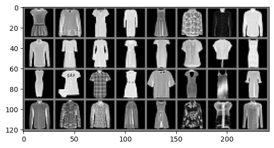
Dress Shirt Dress Dress Dress Shirt Shirt Shirt Shirt Dress Dress Dress Dress Shirt Shirt Dress Dress Dress Shirt Dress Shirt Dress Dress Dress Shirt Shirt Shirt Shirt Dress Shirt Shirt Shirt
A neural network#
Fully connected 1-hidden layer neural network. Flattens the image and treats it as a vector.
Use the methods
nn.Flatten
nn.Linear
nn.init.xavier_normal_
nn.init.zeros_
to build the network
class MLPshallow(nn.Module):
    def __init__(self, hidden_dim=10):
        super().__init__()
        self.hidden_dim = hidden_dim
        self.flatten = nn.Flatten()
        self.l1 = nn.Linear(28 * 28 , self.hidden_dim)
        self.lout = nn.Linear(self.hidden_dim, 1)

        nn.init.xavier_normal_(self.l1.weight)
        nn.init.xavier_normal_(self.lout.weight)

        nn.init.zeros_(self.l1.bias)
        nn.init.zeros_(self.lout.bias)

    def forward(self, x):
        x = self.flatten(x)
        x = F.relu(self.l1(x))
        x = self.lout(x)
        return x

net = MLPshallow(hidden_dim=30)
class MLPshallow(nn.Module):
    def __init__(self, hidden_dim=10):
        super().__init__()
        self.hidden_dim = hidden_dim
        # YOUR CODE HERE

    def forward(self, x):
        # YOUR CODE HERE
        return x

net = MLPshallow(hidden_dim=1000)
The training function#
We train the network with the square loss to predict the class. The labels are normalized to be between \(0\) and \(1\).
i.e. the y-value for images with label i is float(i/9)
Write the training function.
def train(net,
          trainloader,
          N_passes=1,
          lr=0.01):

    optimizer = optim.SGD(net.parameters(), lr=lr)
    criterion = nn.MSELoss()

    losses = []
    i = 0

    for _ in range(N_passes):
        for inputs, labels in trainloader:
            i += 1
            optimizer.zero_grad()

            # print(inputs.shape)
            # print(torch.linalg.vector_norm(inputs, dim=(1, 2, 3)))

            outputs = net(inputs)
            target = labels.float().unsqueeze(1) / 9
            loss = criterion(outputs, target)

            loss.backward()
            optimizer.step()

            losses.append(loss.detach().numpy())

    print(f'Number of gradient steps {i}')

    return losses
def train(net,
          trainloader,
          N_passes=1,
          lr=0.01):

    optimizer = optim.SGD(net.parameters(), lr=lr)
    criterion = nn.MSELoss()

    losses = []
    i = 0

    for _ in range(N_passes):
        for inputs, labels in trainloader:
            i += 1

            #YOUR CODE HERE

            losses.append(loss.detach().numpy())

    print(f'Number of gradient steps {i}')

    return losses
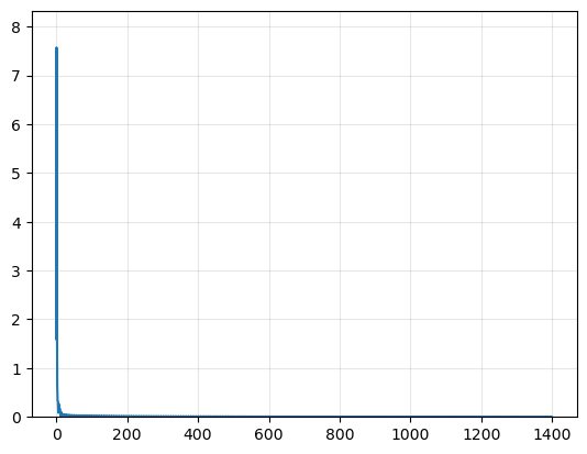
print('Batch size : ', batch_size)

losses = train(net,
    trainloader,
    N_passes=200,
    lr=0.01)

plt.ylim(0, 1.1 * np.max(losses))
plt.plot(losses)
plt.grid(alpha=.3)
Batch size :  32
Number of gradient steps 1400
Checking the training values#
Complete the following function to get the prediction of the network on the data.
Train the network until you interpolate the data.
correct = 0
total = 0
with torch.no_grad():
    for images, labels in trainloader:

        outputs = net(images)
        predicted = c1 + (c2 - c1) * (9 * outputs > (c1 + c2) / 2) # c1 if prediction is less than average,

        total += labels.size(0)
        correct += (predicted.squeeze(1) == labels).sum()

print(f'Accuracy of the network on the {total} train images: {100 * correct // total} %')
Accuracy of the network on the 200 train images: 96 %
correct = 0
total = 0
with torch.no_grad():
    for images, labels in trainloader:

        outputs = net(images)
        predicted = #YOUR CODE HERE

        total += labels.size(0)
        correct += (predicted.squeeze(1) == labels).sum()

print(f'Accuracy of the network on the {total} train images: {100 * correct // total} %')
testloader = torch.utils.data.DataLoader(dset_test, batch_size=8)
dataiter = iter(testloader)
images, labels = next(dataiter)

# print images
imshow(torchvision.utils.make_grid(images[:8]))
print('GrndTruth: ', ' '.join(f'{classes[labels[j]]:5s}' for j in range(8)))

with torch.no_grad():
    outputs = net(images)
    predicted = c1 + (c2 - c1) * (9 * outputs > (c1 + c2) / 2)

    print('Predicted: ', ' '.join(f'{classes[predicted[j]]:5s}' for j in range(8)))
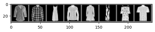
GrndTruth:  Shirt Shirt Dress Shirt Dress Dress Dress Shirt
Predicted:  Shirt Shirt Dress Shirt Shirt Dress Dress Shirt
testloader = torch.utils.data.DataLoader(dset_test, batch_size=8)
dataiter = iter(testloader)
images, labels = next(dataiter)

# print images
imshow(torchvision.utils.make_grid(images[:8]))
print('GrndTruth: ', ' '.join(f'{classes[labels[j]]:5s}' for j in range(8)))

with torch.no_grad():
    outputs = net(images)
    predicted = #YOUR CODE HERE

    print('Predicted: ', ' '.join(f'{classes[predicted[j]]:5s}' for j in range(8)))
Test loss#
correct = 0
total = 0
with torch.no_grad():
    for images, labels in testloader:
        outputs = net(images)
        predicted = c1 + (c2 - c1) * (9 * outputs > (c1 + c2) / 2) # c1 if prediction is less than average,

        total += labels.size(0)
        correct += (predicted.squeeze(1) == labels).sum()

print(f'Accuracy of the network on the {total} test images: {100 * correct // total} %')
Accuracy of the network on the 2000 test images: 88 %
correct = 0
total = 0
with torch.no_grad():
    for images, labels in testloader:
        outputs = net(images)
        predicted = #YOUR CODE HERE

        total += labels.size(0)
        correct += (predicted.squeeze(1) == labels).sum()

print(f'Accuracy of the network on the {total} test images: {100 * correct // total} %')
The NTK#
Let us write the corresponding NTK in the infinite width limit. Use the formula seen in class for the NTK kernel to complete the code below.
class NTK:
    def __init__(self, dset_train):
        self.n = len(dset_train)
        self.train_set = dset_train
        self.train()

    def k(self, x, xprime):
        '''
            NTK Kernel for ReLU with one hidden layer. The delta factor
            is to avoid nan values for arccos(1+eps) from rounding.
        '''
        with torch.no_grad():
            v = torch.linalg.norm(x) * torch.linalg.norm(xprime)
            u = .99999 * torch.dot(x, xprime) / v
            return v * (u * (torch.pi - torch.arccos(u) + torch.sqrt(1 - u ** 2) )/ (2 * np.pi)
                     +  u * (torch.pi - torch.arccos(u)) /  (2 * np.pi))

    def train(self):
        ntrainloader = torch.utils.data.DataLoader(self.train_set, batch_size=self.n)
        dataiter = iter(ntrainloader)
        images, labels = next(dataiter)
        print(images.flatten(start_dim=1, end_dim=3).shape)

        xis = images.flatten(start_dim=1, end_dim=3)
        print(xis.shape)

        self.xis = xis

        # plt.imshow(xis)
        # plt.title('Flattened images')
        # plt.show()

        H = torch.empty((n, n))

        for i in range(n):
            for j in range(n):
                H[i, j] = self.k(xis[i], xis[j])

        # plt.title(f'Gram matrix for {n} x {n} inputs')
        # plt.imshow(H)
        # plt.colorbar()
        # plt.show()

        eigenvalues = np.linalg.eigvalsh(H)
        print(f'Smallest eigenvalue : {eigenvalues[0]}')
        # plt.title('Sorted eigenvalues of the Gram matrix')
        # plt.plot(eigenvalues)
        # plt.grid(alpha=0.3)
        # plt.ylim(0, 1.01 * np.max(eigenvalues))
        # plt.show()

        self.H = H
        self.Hinv = torch.linalg.inv(H)
        self.V =  self.Hinv @ labels.float() / 9

        print(self.V.shape)

        # plt.imshow(V)
        # plt.colorbar()
        # plt.show()

    def apply(self, x):
        s = 0
        for i, xi in enumerate(self.xis):
            s += self.k(x, xi) * self.V[i]
        return s

    def gen_bound(self):
        ntrainloader = torch.utils.data.DataLoader(self.train_set, batch_size=n)
        dataiter = iter(ntrainloader)
        _, labels = next(dataiter)

        return torch.dot(labels.float(), self.Hinv @  labels.float())
class NTK:
    def __init__(self, dset_train):
        self.n = len(dset_train)
        self.train_set = dset_train
        self.train()

    def k(self, x, xprime):
        '''
            NTK Kernel for ReLU with one hidden layer. T
        '''
        delta = .999999
        with torch.no_grad():
            v = torch.linalg.norm(x) * torch.linalg.norm(xprime)
            u = delta * torch.dot(x, xprime) / v
            return # YOUR CODE HERE

    def train(self):
        ntrainloader = torch.utils.data.DataLoader(self.train_set, batch_size=self.n)
        dataiter = iter(ntrainloader)
        images, labels = next(dataiter)
        print(images.flatten(start_dim=1, end_dim=3).shape)

        xis = images.flatten(start_dim=1, end_dim=3)
        print(xis.shape)

        self.xis = xis

        # plt.imshow(xis)
        # plt.title('Flattened images')
        # plt.show()

        H = torch.empty((n, n))

        for i in range(n):
            for j in range(n):
                H[i, j] = self.k(xis[i], xis[j])

        # plt.title(f'Gram matrix for {n} x {n} inputs')
        # plt.imshow(H)
        # plt.colorbar()
        # plt.show()

        eigenvalues = np.linalg.eigvalsh(H)
        print(f'Smallest eigenvalue : {eigenvalues[0]}')
        # plt.title('Sorted eigenvalues of the Gram matrix')
        # plt.plot(eigenvalues)
        # plt.grid(alpha=0.3)
        # plt.ylim(0, 1.01 * np.max(eigenvalues))
        # plt.show()

        self.H = H
        self.Hinv = torch.linalg.inv(H)
        self.V =  self.Hinv @ labels.float() / 9

        print(self.V.shape)

        # plt.imshow(V)
        # plt.colorbar()
        # plt.show()

    def apply(self, x):
        s = 0
        for i, xi in enumerate(self.xis):
            s += self.k(x, xi) * self.V[i]
        return s
ntk = NTK(dset_train)
torch.Size([100, 784])
torch.Size([100, 784])
Smallest eigenvalue : 23.512008666992188
torch.Size([100])
ntk_trainloader = torch.utils.data.DataLoader(dset_train, batch_size=1)

correct_ntk = 0
total = 0
with torch.no_grad():
    for images, labels in ntk_trainloader:
        x = torch.flatten(images.squeeze(0))

        output_ntk = ntk.apply(x)
        predicted_ntk = c1 + (c2 - c1) * (9 * output_ntk > (c1 + c2) / 2) # c1 if prediction is less than average,
        correct_ntk += (predicted_ntk.unsqueeze(0) == labels).numpy()[0]

        total += 1

print(f'Accuracy of NTK on the {total} train images: {100 * correct_ntk // total} %')
Accuracy of NTK on the 100 train images: 100 %
Let us now compare the outputs of the NTK and of the network.
What do you observe? Why?
testloader = torch.utils.data.DataLoader(dset_test)

total = 0
correct_ntk = 0
correct_net = 0
agree = 0

with torch.no_grad():
    for images, labels in testloader:
        x = torch.flatten(images.squeeze(0))

        output_ntk = ntk.apply(x)
        predicted_ntk = c1 + (c2 - c1) * (9 * output_ntk > (c1 + c2) / 2) # c1 if prediction is less than average,
        correct_ntk += (predicted_ntk.unsqueeze(0) == labels).numpy()[0]

        outputs = net(images)
        predicted = c1 + (c2 - c1) * (9 * outputs > (c1 + c2) / 2) # c1 if prediction is less than average,
        correct_net += (predicted.squeeze(1) == labels).numpy()[0]

        # print(labels.shape)
        # print(predicted_ntk.unsqueeze(0).shape, predicted_ntk.unsqueeze(0))
        # print(predicted.squeeze(1).shape, predicted.squeeze(1))

        agree += (predicted_ntk.unsqueeze(0) == predicted.squeeze(1)).numpy()[0]
        total += 1

print(f'Accuracy of NTK on the {total} test images: {100 * correct_ntk // total} %')
print(f'Accuracy of net on the {total} test images: {100 * correct_net // total} %')

print(f'Both methods agree on {100 * agree // total} % of the images')
Accuracy of NTK on the 2000 test images: 91 %
Accuracy of net on the 2000 test images: 86 %
Both methods agree on 89 % of the images
Generalization error#
trainset = datasets.FashionMNIST('../data', train=True, download=True, transform=transform)
r = torch.arange(len(trainset))

bounds = []

n_values = range(100, 2000, 300)

for n in n_values:
    # Build a training set that only contains images with classes c1 and c2, with n / 2 images from each label.

    idxc1 = (torch.as_tensor(trainset.targets) == c1)
    x1 = np.where(np.cumsum(idxc1) == (n / 2))[0][0]
    idxc1 = idxc1 & (r <= x1)

    idxc2 = (torch.as_tensor(trainset.targets) == c2)
    x2 = np.where(np.cumsum(idxc2) == (n / 2))[0][0]
    idxc2 = (torch.as_tensor(trainset.targets) == c2) & (r <= x2)

    idx = idxc1 + idxc2
    dset_train = torch.utils.data.dataset.Subset(trainset, np.where(idx==1)[0])

    ntk = NTK(dset_train)
    bounds.append(ntk.gen_bound())
torch.Size([100, 784])
torch.Size([100, 784])
Smallest eigenvalue : 23.512008666992188
torch.Size([100])
torch.Size([400, 784])
torch.Size([400, 784])
Smallest eigenvalue : 15.195989608764648
torch.Size([400])
torch.Size([700, 784])
torch.Size([700, 784])
Smallest eigenvalue : 13.155244827270508
torch.Size([700])
torch.Size([1000, 784])
torch.Size([1000, 784])
Smallest eigenvalue : 5.420177936553955
torch.Size([1000])
torch.Size([1300, 784])
torch.Size([1300, 784])
Smallest eigenvalue : 5.3553948402404785
torch.Size([1300])
torch.Size([1600, 784])
torch.Size([1600, 784])
Smallest eigenvalue : 5.308578968048096
torch.Size([1600])
torch.Size([1900, 784])
torch.Size([1900, 784])
Smallest eigenvalue : 5.274092197418213
torch.Size([1900])
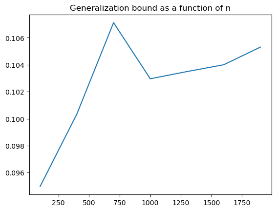
plt.title('Generalization bound as a function of n')
plt.plot(n_values, np.sqrt(bounds / np.array(n_values)))
[<matplotlib.lines.Line2D at 0x147f2fd30>]
The NTK Gram matrix is typically invertible#
if number of data points is smaller than input dim
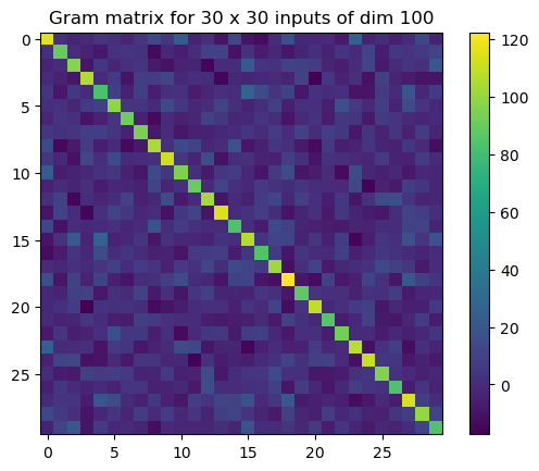
n = 30
d = 100
xis = [torch.randn(d) for _ in range(n)]
# print(xis)
# print(np.dot(xis[n-1], xis[n-1]))
H = torch.empty((n, n))
def k(x, xprime):
with torch.no_grad():
v = torch.linalg.norm(x) * torch.linalg.norm(xprime)
u = .99999 * torch.dot(x, xprime) / v
return v * (u * (torch.pi - torch.arccos(u) + torch.sqrt(1 - u ** 2) )/ (2 * np.pi)
+ u * (torch.pi - torch.arccos(u)) / (2 * np.pi))
for i in range(n):
for j in range(n):
H[i,j] = k(xis[i], xis[j])
plt.title(f'Gram matrix for {n} x {n} inputs of dim {d}')
plt.imshow(H)
plt.colorbar()
plt.show()
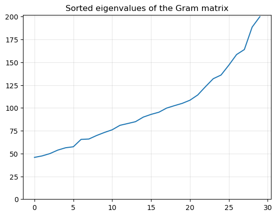
plt.title('Sorted eigenvalues of the Gram matrix')
eigvals = np.linalg.eigvalsh(H)
plt.plot(eigvals)
plt.grid(alpha=0.3)
plt.ylim(0, 1.01 * np.max(eigvals))
plt.show()
# mlp = MLPdeep() # MLPshallow()
# PATH = f'./{dataset.type}_{mlp.net_type}.pth'
# torch.save(mlp.state_dict(), PATH)

# net = MLPdeep() # MLPshallow()
# net.load_state_dict(torch.load(PATH))
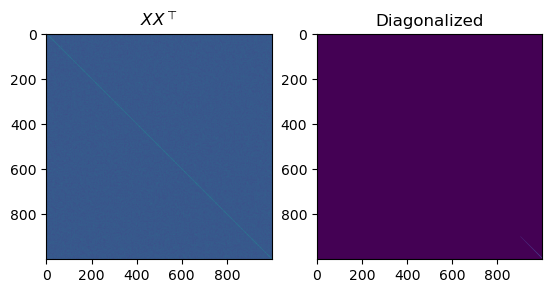
Overparameterized linear regression#
p = 1000
n = 100

X = np.random.normal(size=(p, n))  / np.sqrt(n)
Y = np.random.normal(size=(n, 1))

XXt = X @ X.transpose()
XY = X @ Y

fig, axs = plt.subplots(1, 2)

axs[0].set_title(r'$X X^\top $')
axs[0].imshow(XXt)

eigvals, P = np.linalg.eigh(XXt)
print(rf'Largest eigenvalue of of XX^\top : {max(eigvals)}')

axs[1].set_title('Diagonalized')
axs[1].imshow(P.transpose() @ XXt @ P)
plt.show()

print(np.linalg.matrix_rank(X))
Largest eigenvalue of of XX^\top 16.963392764546683
100
T = 1000
eta = 0.001

ws = np.zeros((T, p, 1))
w = np.random.normal(size=(p, 1))  / np.sqrt(p)

losses = []
for t in range(T):
    w = w - eta * XXt @ w + eta * XY
    ws[t] = w

    losses.append(np.linalg.norm(X.transpose() @ w  - Y)**2 / n )

ws = ws.squeeze(axis=2)
fig, axs = plt.subplots(1, 2, figsize=(16, 4))

axs[0].set_title('Loss')
axs[0].plot(losses)


axs[1].set_title('Relative distance of weights to init')
weight_evol = np.linalg.norm(ws - ws[0, :], axis=1) / np.linalg.norm(ws[0, :])
axs[1].plot(weight_evol, alpha=.5)


plt.show()
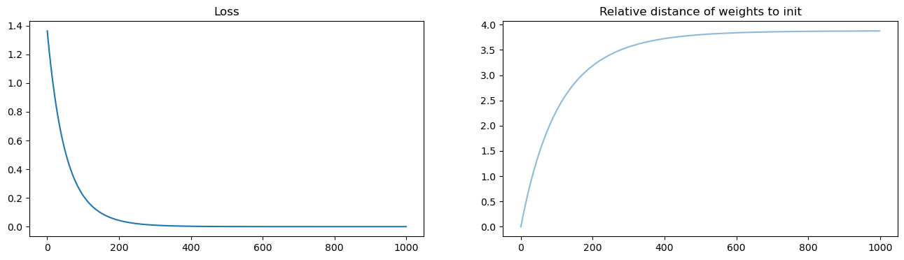
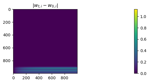
In the right basis, most coordinates of w dont move#
w only moves in a low dimensional subspace: the image of X
fig, ax = plt.subplots(figsize=(40, 3))

plt.title(r'$|w_{t, i} - w_{0, i}|$')
ws_in_base = ws @ P

a = ax.imshow(np.abs((ws_in_base - ws_in_base[0]).transpose()))
fig.colorbar(a)
plt.tight_layout()
plt.show()