TP3 : Lazy training

Observing the lazy training regime with different models

With inspiration from

https://rajatvd.github.io/NTK/

import torch

import torch.optim as optim
import torch.nn as nn
import torch.nn.functional as F

import numpy as np
import matplotlib.pyplot as plt

### Exectutes the script tp3_utils.py which contains code from last time
## Go take a quick look at the functions implemented there

from tp3_utils import * 

# %load_ext autoreload
# %autoreload 2

The data

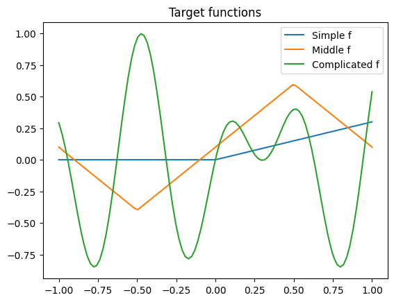
We continue with last week’s toy problem of 1 dimensional regression

xs = np.linspace(-1, 1, 100)
plt.plot(xs, simple_f(xs), label='Simple f')
plt.plot(xs, middle_f(xs), label='Middle f')
plt.plot(xs, complex_f(xs), label='Complicated f')
plt.title('Target functions')
plt.legend()
plt.show()

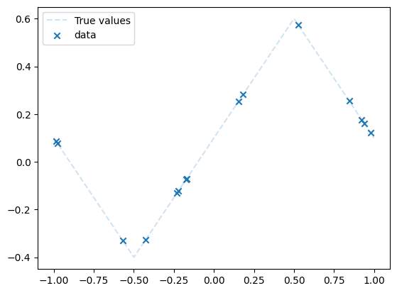
dataset = Data(n=15,
                xmin=-1,
                xmax=1,
                noise_level=0,
                type='middle')

plot_data(dataset)
plt.legend()
plt.show()

The training function

Write the training function

def train(net, 
          dataset, 
          N_steps=1, 
          batch_size=30, 
          lr=0.01, 
          save_weights_every=100):
    
    optimizer = optim.SGD(net.parameters(), lr=lr)
    criterion = nn.MSELoss()

    losses = []
    weights = []

    for i in range(N_steps): 
        inputs, labels= dataset.next_batch(batch_size)
        optimizer.zero_grad()

        outputs = net(inputs)
        loss = criterion(outputs, labels)
        
        loss.backward()
        optimizer.step()

        losses.append(loss.detach().numpy())

        if i % save_weights_every == 0 and (save_weights_every > 0):
            with torch.no_grad():
                weights.append(net.save_weights())

    return losses

def train(net, 
          dataset, 
          N_steps=1, 
          batch_size=30, 
          lr=0.01, 
          save_weights_every=100):
    
    # YOUR CODE HERE

    losses = []
    weights = []

    for i in range(N_steps): 
        # YOUR CODE HERE

        losses.append(loss.detach().numpy())

        if i % save_weights_every == 0 and (save_weights_every > 0):
            with torch.no_grad():
                weights.append(net.save_weights())

    return losses

Test your training

model = MLPdeep(hidden_dim=10)
losses = train(model, 
                dataset, 
                N_steps=10000, 
                batch_size=15, 
                lr=.1, 
                save_weights_every=1,
                )

plot_net(model)
plot_data(dataset)
plt.show()

plt.plot(losses)
plt.show()

---------------------------------------------------------------------------
NameError                                 Traceback (most recent call last)
Cell In[6], line 2
      1 model = MLPdeep(hidden_dim=10)
----> 2 losses = train(model, 
      3                 dataset, 
      4                 N_steps=10000, 
      5                 batch_size=15, 
      6                 lr=.1, 
      7                 save_weights_every=1,
      8                 )
     10 plot_net(model)
     11 plot_data(dataset)

Cell In[5], line 16, in train(net, dataset, N_steps, batch_size, lr, save_weights_every)
     11 weights = []
     13 for i in range(N_steps): 
     14     # YOUR CODE HERE
---> 16     losses.append(loss.detach().numpy())
     18     if i % save_weights_every == 0 and (save_weights_every > 0):
     19         with torch.no_grad():

NameError: name 'loss' is not defined

A linear model

We define a family of linear models with sinusoidal features. The feature map is

\[ \phi(x) = ( \cos(2 \pi x) , \sin(2 \pi x), \cos(4 \pi x) , \sin(4 \pi x), \dots , \cos(2k \pi x) , \sin(2k \pi x)) \]

where \(k\) is feature_dim / 2.

class LinSin(nn.Module): 
    """
        A linear model with sinusoidal features. Assumes feature_dim is even.
    """
    def __init__(self, feature_dim): 
        super().__init__()
        self.feature_dim = feature_dim
        self.lout = nn.Linear(self.feature_dim, 1)

        self.weight_history = []

    def phi(self, x):
        """
            Computes $sin(2\pi k x), cos(2\pi k x) $ for k in $[feature_dim / 2]$
        """
        r = 2 * np.pi * torch.arange(int(self.feature_dim / 2)) * x
        return torch.concatenate([torch.sin(r), torch.cos(r)], axis=1)

    def save_weights(self): 
        with torch.no_grad():
            l = list(self.parameters())
            self.weight_history.append(np.copy(l[-1].numpy()))

    def forward(self, x): 
        return self.lout(self.phi(x))

class LinSin(nn.Module): 
    """
        A linear model with sinusoidal features
    """
    def __init__(self, feature_dim): 
        super().__init__()
        self.feature_dim = feature_dim
        self.lout = nn.Linear(self.feature_dim, 1)

        self.weight_history = []

    def phi(self, x):
        """
            Computes $sin(2\pi k x), cos(2\pi k x) $ for k in $[feature_dim / 2]$
        """
        # YOUR CODE HERE
        pass

    def save_weights(self): 
        with torch.no_grad():
            l = list(self.parameters())
            self.weight_history.append(np.copy(l[-1].numpy()))

    def forward(self, x): 
        # YOUR CODE HERE
        pass

Test the linear model

model = LinSin(feature_dim=8)
losses = train(model, 
                dataset, 
                N_steps=10000, 
                batch_size=15, 
                lr=.01, 
                save_weights_every=1,
                )

plot_net(model)
plot_data(dataset)
plt.show()

fig, axs = plt.subplots(1, 2, figsize=(12, 4))
axs[0].loglog(losses)
axs[0].set_title('Train loss')

all_weights1 = np.array(model.weight_history)
weight_evol = np.linalg.norm(all_weights1 - all_weights1[0], axis=1) / np.linalg.norm(all_weights1[0])
axs[1].plot(weight_evol, alpha=.5) 
axs[1].set_title('Relative weight movement of last layer')

Text(0.5, 1.0, 'Relative weight movement of last layer')

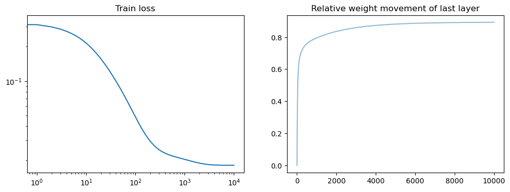
Question: what do the plots mean?

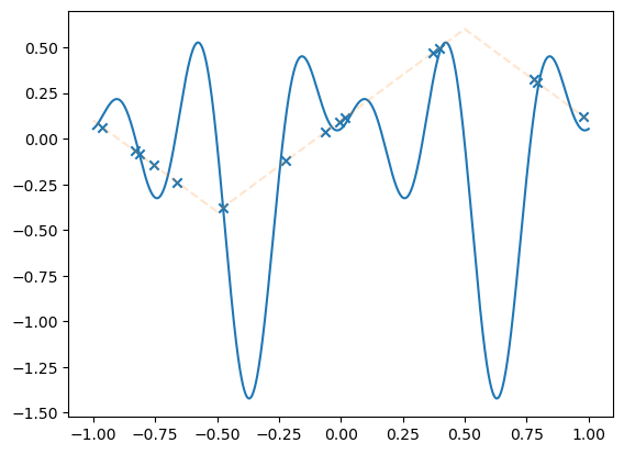
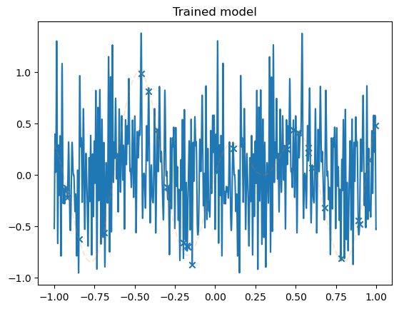
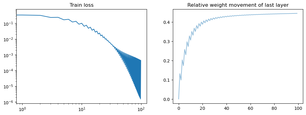
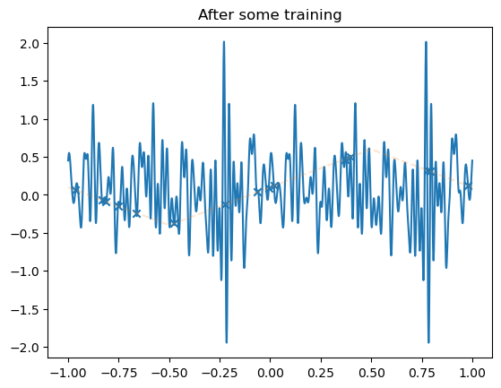
Let us now repeat the code above with a large feature dimension. What you do observe?

model = LinSin(feature_dim=200)
losses = train(model, 
                dataset, 
                N_steps=100, 
                batch_size=15, 
                lr=.01, 
                save_weights_every=1,
                )

plot_net(model)
plot_data(dataset)
plt.title('Trained model')
plt.show()

fig, axs = plt.subplots(1, 2, figsize=(12, 4))
axs[0].loglog(losses)
axs[0].set_title('Train loss')

all_weights1 = np.array(model.weight_history)
weight_evol = np.linalg.norm(all_weights1 - all_weights1[0], axis=1) / np.linalg.norm(all_weights1[0])
axs[1].plot(weight_evol, alpha=.5) 
axs[1].set_title('Relative weight movement of last layer')

plt.show()

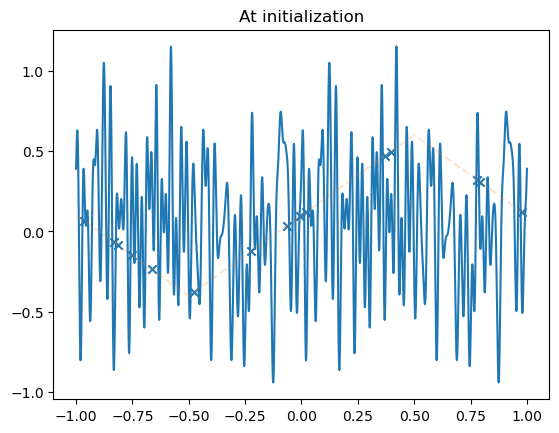
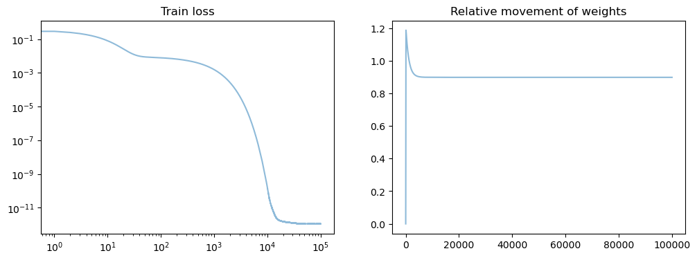
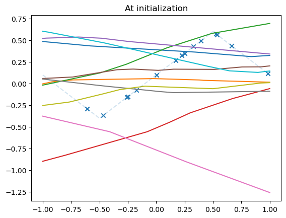
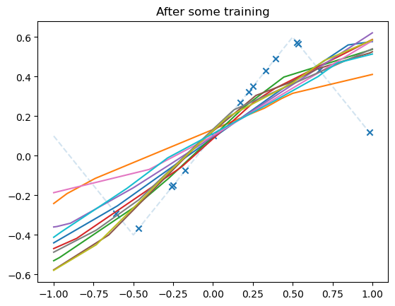
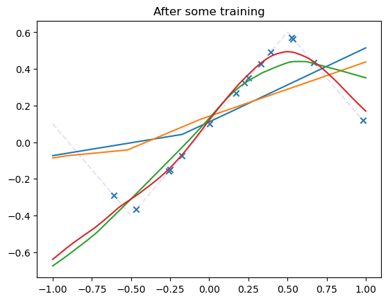
Robustness of fast convergence for linear models

Run 10 instances of the linear model with different initializations.

Are there significant differences between the models?

model_list = []
N_models = 1
for _ in range(N_models): 
    model = LinSin(feature_dim=100)
    model_list.append(model)
    plot_net(model)

plot_data(dataset)
plt.title('At initialization')

all_losses = [[] for _ in range(N_models)]
all_weights = []

N_steps = 100000

for i, model in enumerate(model_list):
    losses = train(model, 
                   dataset, 
                   N_steps=N_steps, 
                   batch_size=30, 
                   lr=.01, 
                   save_weights_every=1,
                   )
    all_losses[i] += losses
    plot_net(model)

plot_data(dataset)
plt.title('After some training')

plt.show()

fig, axs = plt.subplots(1, 2, figsize=(12, 4))

axs[0].set_title('Train loss')
for losses in all_losses:
    points = np.arange(0, len(losses), 1)  
    losses = np.array(losses)
    axs[0].loglog(points, losses[points], alpha=.5)

axs[1].set_title('Relative movement of weights')
for model in model_list:    
    all_weights1 = np.array(model.weight_history)
    weight_evol = np.linalg.norm(all_weights1 - all_weights1[0], axis=1) / np.linalg.norm(all_weights1[0])

    axs[1].plot(weight_evol, alpha=.5) 

plt.show()

Lazy training of non-linear models

We now train some neural nets in different regimes and try to see when lazy training occurs.

Question How are nets initialized in pytorch?

model_list = []
N_models = 10
for _ in range(N_models): 
    model = MLPshallow(hidden_dim=10)
    model_list.append(model)
    plot_net(model)

plot_data(dataset)
plt.title('At initialization')

all_losses = [[] for _ in range(N_models)]
all_weights = []

N_steps = 5000

for i, model in enumerate(model_list):
    losses = train(model, 
                   dataset, 
                   N_steps=N_steps, 
                   batch_size=30, 
                   lr=.001, 
                   save_weights_every=1,
                   )
    all_losses[i] += losses
    plot_net(model)

plot_data(dataset)
plt.title('After some training')

plt.show()

fig, axs = plt.subplots(1, 2, figsize=(12, 4))

axs[0].set_title('Train loss')
for losses in all_losses:
    points = np.arange(0, len(losses), 1)  
    losses = np.array(losses)
    axs[0].loglog(points, losses[points], alpha=.5)

axs[1].set_title('Relative weight movement of last layer')
for model in model_list:    
    all_weights1 = np.array(model.weight_history)
    weight_evol = np.linalg.norm(all_weights1 - all_weights1[0], axis=1) / np.linalg.norm(all_weights1[0])

    axs[1].plot(weight_evol, alpha=.5) 

plt.show()

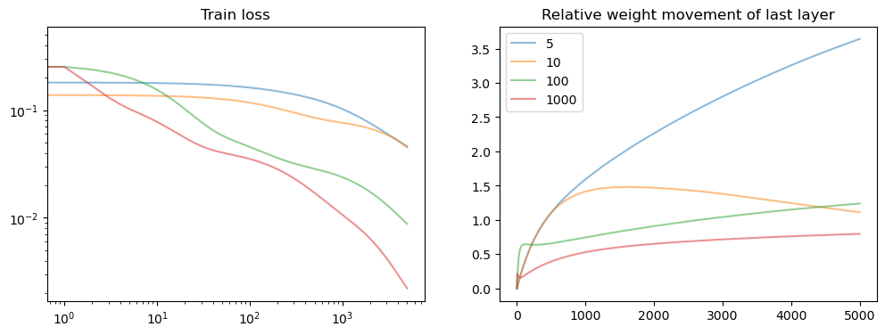
Thin vs. Wide networks

Let us now vary the width of our network. What happens?

model_list = []

width_list = [5, 10, 100, 1000]

for width in width_list: 
    model = MLPshallow(hidden_dim=width)
    model_list.append(model)
    plot_net(model, label=f'Width = {model.hidden_dim}')

plot_data(dataset)
plt.title('At initialization')
plt.legend()

all_losses = [[] for _ in width_list]
all_weights = []

N_steps = 5000

for i, model in enumerate(model_list):
    losses = train(model, 
                   dataset, 
                   N_steps=N_steps, 
                   batch_size=30, 
                   lr=.001, 
                   save_weights_every=1,
                   )
    all_losses[i] += losses
    plot_net(model, label=f'Width = {model.hidden_dim}')

plot_data(dataset)
plt.title('After some training')

plt.show()

fig, axs = plt.subplots(1, 2, figsize=(12, 4))

axs[0].set_title('Train loss')
for i, losses in enumerate(all_losses):
    points = np.arange(0, len(losses), 1)  
    losses = np.array(losses)
    axs[0].loglog(points, losses[points], alpha=.5, label=f'{width_list[i]}')

axs[1].set_title('Relative weight movement of last layer')
for model in model_list:    
    all_weights1 = np.array(model.weight_history)
    weight_evol = np.linalg.norm(all_weights1 - all_weights1[0], axis=1) / np.linalg.norm(all_weights1[0])

    axs[1].plot(weight_evol, alpha=.5, label=f'{model.hidden_dim}') 

plt.legend()
plt.show()

Bad initialization can you get you out of the Lazy regime

We simulate bad initialization by taking two steps of gradient descent from initialization.

model_list = []
N_models = 10
for _ in range(N_models): 
    model = MLPshallow(hidden_dim=100)
    model_list.append(model)
    train(model, 
        dataset, 
        N_steps=2, 
        batch_size=30, 
        lr=1, 
        save_weights_every=-1,
        )
    plot_net(model)


plot_data(dataset)
plt.title('At bad initialization')

all_losses = [[] for _ in range(N_models)]
all_weights = []

N_steps = 1000
xmin = np.min(dataset.inputs.detach().numpy())
xmax = np.max(dataset.inputs.detach().numpy())
plt.xlim(xmin, xmax)
print(xmin, xmax)

for i, model in enumerate(model_list):
    losses = train(model, 
                   dataset, 
                   N_steps=N_steps, 
                   batch_size=30, 
                   lr=.001, 
                   save_weights_every=1,
                   )
    all_losses[i] += losses
    plot_net(model, xmin=xmin, xmax=xmax)

plot_data(dataset)
plt.title('After some training')

plt.show()

fig, axs = plt.subplots(1, 2, figsize=(12, 4))

axs[0].set_title('Train loss')
for i, losses in enumerate(all_losses):
    points = np.arange(0, len(losses), 1)  
    losses = np.array(losses)
    axs[0].loglog(points, losses[points], alpha=.5)

axs[1].set_title('Relative weight movement of last layer')
for model in model_list:    
    all_weights1 = np.array(model.weight_history)
    weight_evol = np.linalg.norm(all_weights1 - all_weights1[0], axis=1) / np.linalg.norm(all_weights1[0])

    axs[1].plot(weight_evol, alpha=.5) 

plt.show()

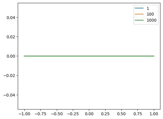
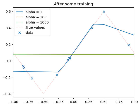
Scaling

Now we attempt to enter the lazy regime by scaling the model outputs.

n_points = 10

dataset = Data(n=n_points,
                xmin=-1,
                xmax=1,
                noise_level=0,
                type='middle')

class ScaledModel(MLPdeep):
    """"
        From a base network, creates a scaled copy with 0 initialization. Keeps a frozen copy of a base model. 

        alpha: scaling factor
    """
    def __init__(self, base_model, alpha=1):
        super().__init__(hidden_dim=base_model.hidden_dim)
        
        self.alpha = alpha
        self.load_state_dict(base_model.state_dict())

        self.base_model = [base_model] # trick to hide from the other parameters dictionary. Probably not the proper way to do this...

    def forward(self, x):
        """
            Scales the output and subtracts the initial function 
        """
        with torch.no_grad():
            base = self.base_model[0].forward(x).detach()
        return self.alpha * (super().forward(x) - base)

base_model = MLPdeep(hidden_dim=8)

alphas = [1, 100, 1000]#, 2000, 10000]
model_list = []

for alpha in alphas: 
    new_model = ScaledModel(base_model, alpha=alpha)
    new_model.load_state_dict(base_model.state_dict())
    model_list.append(new_model)

    plot_net(new_model, label=f'{alpha}')

all_losses = [[] for _ in range(len(model_list))]

plt.legend()
plt.show()

train(model_list[2], 
    dataset, 
    N_steps=10000,
    batch_size=n_points, 
    lr=.1 / alphas[2]**2, 
    save_weights_every=1,
    )

plot_data(dataset)
plt.legend()
plt.title('After some training')


for i, model in enumerate(model_list):
    plot_net(model, xmin=xmin, xmax=xmax, label=f'alpha = {alphas[i]}')

N_steps = 10000
xmin = -1 #np.min(dataset.inputs.detach().numpy())
xmax = 1 #np.max(dataset.inputs.detach().numpy())
plt.xlim(xmin, xmax)
print(xmin, xmax)

for i, model in enumerate(model_list):
    losses = train(model, 
                   dataset, 
                   N_steps=N_steps,
                   batch_size=n_points, 
                   lr=.01 / alphas[i]**2 , 
                   save_weights_every=1,
                   )
    all_losses[i] += losses 
    plot_net(model, xmin=xmin, xmax=xmax, label=f'alpha = {alphas[i]}')

plot_data(dataset)
plt.legend()
plt.title('After some training')

plt.show()

-1 1

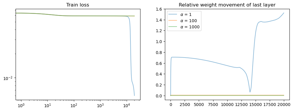
fig, axs = plt.subplots(1, 2, figsize=(12, 4))

axs[0].set_title('Train loss')
for i, losses in enumerate(all_losses):
    points = np.arange(0, len(losses), 1)  
    losses = np.array(losses) # / alphas[i] ** 2
    axs[0].loglog(points, losses[points], alpha=.5, label=f'{alphas[i]}')

axs[1].set_title('Relative weight movement of last layer')
for i, model in enumerate(model_list):    
    all_weights1 = np.array(model.weight_history)
    weight_evol = np.linalg.norm(all_weights1 - all_weights1[0], axis=1) / np.linalg.norm(all_weights1[0])

    axs[1].plot(weight_evol, alpha=.5, label=rf'$\alpha$ = {alphas[i]}')

plt.legend()
plt.show()

5 - The effect of scaling on a 1D model

Question Explain the piece of code below.

see blog post

import numpy as np
import matplotlib.pyplot as plt

w_0 = 1.5

def f(x, w): 
    return w * x /2  +  np.log(1 + w**2) * x / 5  + .1 * np.sin(np.exp(2*w))#np.exp(0.1*w))

def h(x, w, w_0=.4): 
    return f(x, w) * (w - w_0)

def linh(x, w, w_0=.4):
    return  f(x, w_0) * (w - w_0)

xys = [(1.5, 3)]

def l(w, alpha): 
    return np.sum([(alpha * h(x, w, w_0=w_0) - y) ** 2 / 2 for x, y in xys]) / alpha ** 2

def linl(w, alpha):
    return np.sum([(alpha * linh(x, w, w_0=w_0) - y) ** 2 / 2 for x, y in xys]) / alpha ** 2

alphas = [1, 5, 10, 50,  100, 1000, 2000, 10000]

ws = np.linspace(-1, 1, 100)
plt.title('h(2; w)')
plt.plot(ws, [h(2, w, w_0=w_0) for w in ws])
plt.show()

for alpha in alphas:
    delta = 2 / alpha ** (3/4)
    ws = np.linspace(w_0 - delta, w_0 + delta, 5000)
    plt.title(f'Loss landscape of scaled model: alpha = {alpha}')
    plt.plot(ws, [l(w, alpha) for w in ws], label='Loss of scaled model')
    plt.plot(ws, [linl(w, alpha) for w in ws], label='Loss of scaled linearized model')
    plt.grid(alpha=.2)
    plt.legend()
    plt.show()

import numpy as np
import matplotlib.pyplot as plt

w_0 = 1.5

def f(x, w): 
    return w * x /2  +  np.log(1 + w**2) * x / 5  + .1 * np.sin(np.exp(2*w))

def h(x, w, w_0=.4): 
    return f(x, w) * (w - w_0)

def linh(x, w, w_0=.4):
    return  f(x, w_0) * (w - w_0)

xys = [(1.5, 3)]

def l(w, alpha): 
    return np.sum([(alpha * h(x, w, w_0=w_0) - y) ** 2 / 2 for x, y in xys]) / alpha ** 2

def linl(w, alpha):
    return np.sum([(alpha * linh(x, w, w_0=w_0) - y) ** 2 / 2 for x, y in xys]) / alpha ** 2

alphas = [1, 5, 10, 50,  100, 1000, 2000, 10000]

for alpha in alphas:
    delta = 2 / alpha ** (3/4)
    ws = np.linspace(w_0 - delta, w_0 + delta, 5000)
    plt.title(f'??: alpha = {alpha}')
    plt.plot(ws, [l(w, alpha) for w in ws], label='??')
    plt.plot(ws, [linl(w, alpha) for w in ws], label='??')
    plt.grid(alpha=.2)
    plt.legend()
    plt.show()

Pieces

mlp = model_list[0]

for name, param in mlp.named_parameters(): 
    print(name)
    print(param.shape)
    print(np.linalg.norm((param.detach().numpy())))

a = np.arange(10,30)
shifted_a = np.zeros(20)
print(shifted_a)
shifted_a[1:] = a[:-1]
print(shifted_a)
print(a)

evol = (a - shifted_a)[1:] / a[1:]
print(evol)

plt.title('Difference in succesive weights')
for model in model_list:    
    all_weights1 = np.array(model.weight_history)
    shifted_weights = np.zeros(all_weights1.shape)
    shifted_weights[1:, :] = all_weights1[:-1, :]
    weight_evol = (np.linalg.norm((all_weights1 - shifted_weights)[1:], axis=1) 
                   / np.linalg.norm(all_weights1[1:], axis=1))

    plt.plot(weight_evol, alpha=.5) 


plt.show()

You can use the following code snippet to save your network.

# mlp = MLPdeep() # MLPshallow()
# PATH = f'./{dataset.type}_{mlp.net_type}.pth'
# torch.save(mlp.state_dict(), PATH)

# net = MLPdeep() # MLPshallow()
# net.load_state_dict(torch.load(PATH))

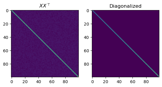
p = 100
n = 5000

X = np.random.normal(size=(p, n))  / np.sqrt(n) 
Y = np.random.normal(size=(n, 1))

XXt = X @ X.transpose()
XY = X @ Y

fig, axs = plt.subplots(1, 2)

axs[0].set_title(r'$X X^\top $')
axs[0].imshow(XXt)

eigvals, P = np.linalg.eigh(XXt)
print(max(eigvals))

axs[1].set_title('Diagonalized')
axs[1].imshow(P.transpose() @ XXt @ P)
plt.show()

print(np.linalg.matrix_rank(X))

1.2872850938240181

100

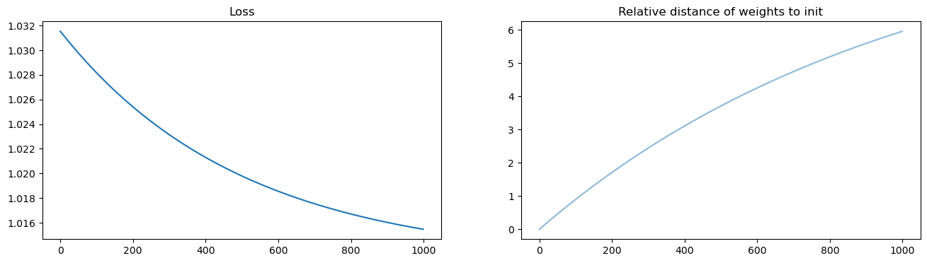
T = 1000
eta = 0.001

ws = np.zeros((T, p, 1))
w = np.random.normal(size=(p, 1))  / np.sqrt(p)

losses = []
for t in range(T):
    w = w - eta * XXt @ w + eta * XY
    ws[t] = w

    losses.append(np.linalg.norm(X.transpose() @ w  - Y)**2 / n )

ws = ws.squeeze(axis=2)
fig, axs = plt.subplots(1, 2, figsize=(16, 4))

axs[0].set_title('Loss')
axs[0].plot(losses) 


axs[1].set_title('Relative distance of weights to init')
weight_evol = np.linalg.norm(ws - ws[0, :], axis=1) / np.linalg.norm(ws[0, :])
axs[1].plot(weight_evol, alpha=.5) 
 

plt.show()

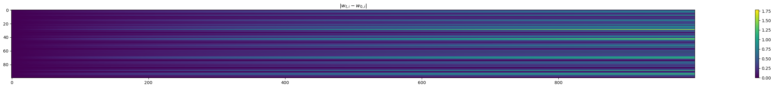
In the right basis, most coordinates of w dont move

w only moves in a low dimensional subspace: the image of X

fig, ax = plt.subplots(figsize=(40, 3))

plt.title(r'$|w_{t, i} - w_{0, i}|$')
ws_in_base = ws @ P

a = ax.imshow(np.abs((ws_in_base - ws_in_base[0]).transpose()))
fig.colorbar(a)
plt.tight_layout()
plt.show()

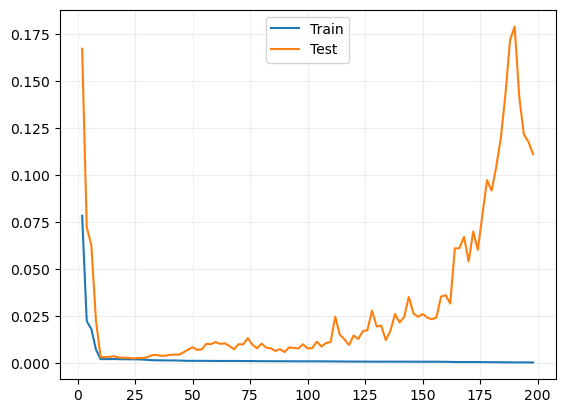
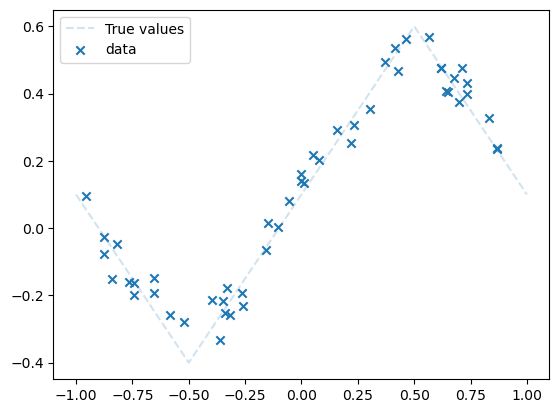
Bias complexity tradeoff

xs = np.linspace(-1, 1, 100)
plt.plot(xs, simple_f(xs), label='Simple f')
plt.plot(xs, middle_f(xs), label='Middle f')
plt.plot(xs, complex_f(xs), label='Complicated f')
plt.title('Target functions')
plt.legend()
plt.show()

npoints = 50

dataset = Data(n=npoints,
                xmin=-1,
                xmax=1,
                noise_level=0.05,
                type='middle')

plot_data(dataset)
plt.legend()
plt.show()

class LinSin(nn.Module): 
    """
        A linear model with sinusoidal features. Assumes feature_dim is even.
    """
    def __init__(self, feature_dim): 
        super().__init__()
        self.feature_dim = feature_dim
        self.lout = nn.Linear(self.feature_dim, 1)

        self.weight_history = []

    def phi(self, x):
        """
            Computes $sin(2\pi k x), cos(2\pi k x) $ for k in $[feature_dim / 2]$
        """
        r = .2 * np.pi * torch.arange(int(self.feature_dim / 2)) * x
        return torch.concatenate([torch.sin(r), torch.cos(r)], axis=1)

    def save_weights(self): 
        with torch.no_grad():
            l = list(self.parameters())
            self.weight_history.append(np.copy(l[-1].numpy()))

    def forward(self, x): 
        return self.lout(self.phi(x))

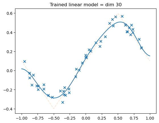
model = LinSin(feature_dim=30)
losses = train(model, 
                dataset, 
                N_steps=2000, 
                batch_size=npoints, 
                lr=.01, 
                save_weights_every=-1,
                )

plot_net(model)
plot_data(dataset)
plt.title('Trained linear model = dim 30')
plt.show()

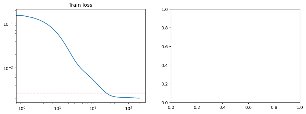
fig, axs = plt.subplots(1, 2, figsize=(12, 4))
axs[0].loglog(losses)
axs[0].set_title('Train loss')
true_risk = dataset.risk(model)
print(true_risk)
axs[0].axhline(true_risk, color='red', alpha=.5, linestyle='--')


plt.show()

tensor(0.0026)

# train_losses = []
# var_train = []
# risks = []
dimensions = np.array(list(range(150, 200, 2)))# + list(range(100, 300, 2)))
for dim in dimensions:
    losses = []
    local_risks = []
    for _ in range(10):
        model = LinSin(feature_dim=dim)
        losses.append(train(model, 
                        dataset, 
                        N_steps=1000, 
                        batch_size=100, 
                        lr=.1, 
                        save_weights_every=-1,
                        )[-1])
        local_risks.append(dataset.risk(model).detach())
    train_losses.append(np.mean(losses))
    var_train.append(np.var(losses))
    risks.append(np.mean(local_risks))
    

plt.grid(alpha=.2)

plt.plot(np.arange(2, 200, 2),train_losses, label='Train')
plt.plot(np.arange(2, 200, 2), risks, label='Test')
plt.legend()

<matplotlib.legend.Legend at 0x29090d610>